Still Looking for Salt...and automated methods to map it

I continue my work on detecting salt domes on Axel Heiberg using satellite imagery. Today I will write about a new technique I learned, which turned out to highlight salt domes very nicely - Principal Component Analysis (PCA).
PCA eliminates redundancy, condensing attribute variability into a fewer number of bands.
For details on the concepts behind Principal Component transformation check out the ArcMap help: http://desktop.arcgis.com/en/arcmap/latest/tools/spatial-analyst-toolbox/how-principal-components-works.htm
(another website which explains PCA and eigenvalues/vectors very clearly: https://georgemdallas.wordpress.com/2013/10/30/principal-component-analysis-4-dummies-eigenvectors-eigenvalues-and-dimension-reduction/).

I used the Principal Components Tool (Spatial Analyst) in ArcMap on the full Landsat 8 mosaic of Axel Heiberg Island, which consisted of 6 bands (band 2-7). The output of this transformation is a multi-band raster:

PC1:	PC2:	PC3:
PC4: Salt is very bright	PC5: Noisy	PC6: No information

(I applied an ice mask)

After PC transformation most of the information is contained within the first four bands, instead of six. I can see that in PC band 4 salt domes have very high attribute values, and thus are very bright. 

The color composite: R:4 G:3 B:2 highlights the salt domes in bright yellow, thus both PC bands 4 and 3 have very high values, while band 2 has very low values. Figure below is a subset of the PCA 432 color composite.

Landsat 8 PCA:432

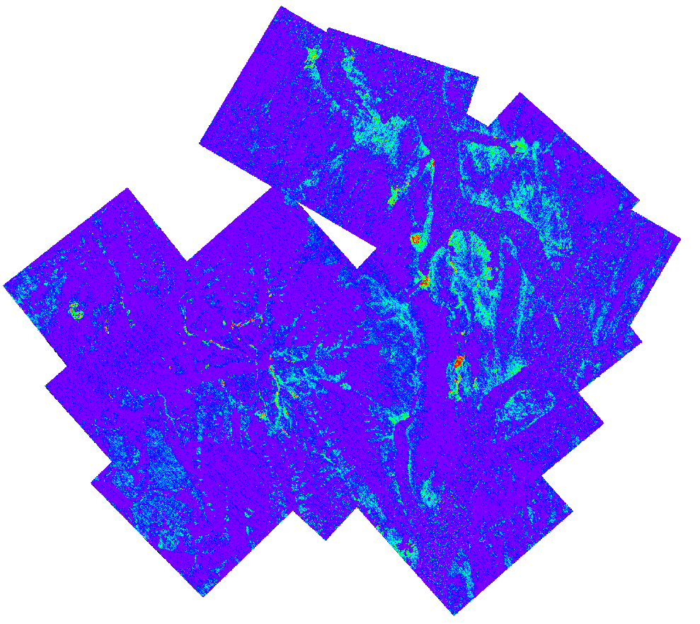
The same transformation was done to the ASTER TIR (thermal) mosaic: 

ASTER: TIR: PCA: 132

The salt domes have a bright "beet" color. 

Next step is to find a convenient automated method to map the salt. Before I did it manually: created a new shapefile and traced salt domes one by one. This method is good but timeconsuming, moreover, the outcome is highly dependent on the accuracy of the mapper. 

The new method I tried is a Supervised Image Classification. 

ASTER: TIR: Training Samples

First I had to create training samples. I decided to have just three classes: salt, ice/water and not salt (all other surfaces). After training samples are collected ArcMap allows us to create a signature file, which contains spectral signatures of all the classes in the multidimensional space, thus all bands included in the raster are analyzed. To avoid confusion, before collecting training samples and creating a signature file, I used a Make Raster Layer Tool (Data Management) to isolate only the PC bands which contained useful information (PC: 1,3 and 2). 

This way information only from PC bands 1, 3 and 2 was included in the signature file. The next step is to use this signature in the Maximum Likelihood Classification Tool (MLC). MLC assumes that distribution of the attribute values is normal in the multidimensional space (number of dimensions is equal to the number of bands). The algorithm behind the tool calculates statistical probability for each class to include a given cell based on its position in the feature (attribute) space and assigns it to the class which has the highest probability. For more information on how the MLC works check out the ArcMap help section: http://desktop.arcgis.com/en/arcmap/10.3/tools/spatial-analyst-toolbox/how-maximum-likelihood-classification-works.htm

When using the MLC tool there are two inputs: raster file (ASTER TIR PCA) and a signature file, created in the previous step. To get rid of noise I applied a Majority Filter Tool to the classification result. The final classified raster is shown below. 

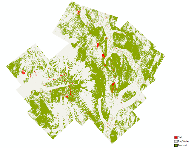
ASTER: TIR: Supervised Maximum Likelihood Classification

I think this mapping experiment was very successful. Not in all cases it can be substituted for the manual mapping, but sometimes it can be very handy.  

Spectral Signature Extraction (SWIR)

Last week I wrote about Spectral Signature Extraction from TIR or thermal infra-red imagery, this week I will continue Spectral Signature Extraction but this time from the SWIR or short wave infra-red imagery of the same area (Axel Heiberg Island).

I went through the same procedure as last time.
First I drew ten ROIs or regions of interest based on the color of the SWIR R: Band 4 (1.60-1.70 micrometers), G: Band 6 (2.185-2.225 micrometers), B: Band 8 (2.295-2.365 micrometers) color composite. I chose magenta regions assuming that they should represent salt domes (as show in the images below).
   

In order to compare salt domes with each other I visualized their spectra in one graph with the help of ENVI 5.3 software.

The bottom three spectra (# 5, 3 and 2) look at little bit different from the rest of the spectra as first I tried to use the same regions of interest which were created based on the TIR image, however it did not work very well as some shaded areas got included. Otherwise all the spectra look very similar.

Next step is to compare the obtained spectra to the Spectral Libraries. I used a Spectral Library included in the ENVI software called aster_mineral_usgs_perknic_2756. However, this Spectral Library is designed for hyperspectral imagery and in order to be used for multispectral data it has to be resampled. I used the tool called Spectral Resampling in order to resample the spectral library to the wavelength range I am interested in, which is 1.60 - 2.43 micrometer, and a necessary number of bands (SWIR ASTER data consists of 6 spectral bands).

Once the mineral library was resampled I could run Spectral Analyst tool to compare my spectra to the library spectra. These are results for some of the salt domes (gypsum was always first on the list):

 


Spectral Analyst confirmed that the areas highlighted as magenta in the SWIR imagery are indeed salt domes composed of gypsum.

When I was analyzing TIR (thermal infra-red) imagery it was unclear whether we are dealing with anhydrite (CaSO₄) or gypsum (CaSO₄.2H₂O) because their spectra are very close in the thermal range, however, in short wave infra-red it is easier to distinguish between the two as shown in the figure below (red frame) (Bishop, 2014):


References:
Bishop, J., Lane, M., Byar, M., King, S., Brown, A., & Swayze, G. (2014). Spectral properties of ca-sulfates: Gypsum, bassanite, adn anhydrite. American Mineralogist, 99(10), 2105-2115. doi:10.2138/am-2014-4756

Spectral Signature Extraction

For the last two weeks I have been learning to extract spectral signatures from ASTER TIR (thermal infra-red 8.125 - 11.650 micrometers) imagery and compare these signatures to the already existing spectral libraries. This comparison allows to identify what rock type or even more specifically what mineral we are looking at.

Today I will write about comparing spectral signatures extracted from different salt diapirs among themselves. This was done in order to compare how similar salt domes are, as well as to compare them to the spectral responses found in spectral libraries.

First of all I created 9 Regions of Interest or ROIs in ENVI 5.3. In order to choose most representative pixels within each dome I created a grey scale ratio: (band 10 + band 12 + band 13)/ band 11 (Dr. Livio Tornabene found that this ratio is the best for highlighting salt domes). Then a rainbow color table was applied to this ratio as well as a little bit of stretching as illustrated below.

 

ASTER TIR: (b10+b12+b13)/b11 + rainbow color table



  

This manipulation allowed me to highlight most representative pixels of the salt domes in red color.
If we look at the TIR (12 11 13) image we can see that the salt domes stand out in red or magenta, however, they all have different tinges, so choosing domes for my regions of interest I tried to incorporate all different shades of magenta to see if their spectra differ.
The image below on the right is a thermal  infra-red image of a section of Axel Heiberg Island with all the regions of interest marked by numbers 1- 9. And the image below on the left illustrates one of the ROIs which was drawn on the biggest salt dome of Axel Heiberg.

ASTER TIR: R:b12 G:b11 B:b13

 

Round Salt Dome ROI (most representative pixels)

Once all the nine ROIs were chosen I was able visualize them all on one graph allowing the comparison of the mean values of each of the five bands for each region of interest.



Just looking at the graph above I can see that most of the spectra have a very similar shape.There is a deep absorption feature in band 11 (second band of the TIR) and this is where most variability occurs. Only two regions of interest had a different shape of spectra: # 1 and #9, in spite of the fact that they also were highlighted as magenta in the TIR image.

Next step is running Spectral Analyst tool in order to compare our spectra to the spectral libraries.
I used two spectral libraries: ASUs_wasrds_rocks to ASTER TIR for identifying rock types and ASU mineral ASTER TIR for mineral identification created by the Arizona State University.

Comparing spectral signatures of #1 and #9 to the rock library showed that they are not similar to Rock Gypsum, but resemble much more the spectrum of Arkose (type of sandstone - silica rich) as illustrated below.


Comparison of all other ROIs to the rock spectral libraries produced the following results: Rock Gypsum or Rock Anhydrite as shown below.


While comparison to the mineral libraries gave the following results: Gypsum or Gypsum var. Alabaster.


Of course this method is not very precise as the spectral resolution of ASTER images is 90m, however, it is a good approximation and it proves that the areas highlighted in magenta on the TIR ASTER images are indeed salt domes and are more specifically, most likely, gypsum.

Masking

Today I will talk about a new technique I have learned - masking.

Not all the surfaces present in a remotely sensed image are useful for our analysis. In the case of Axel Heiberg, there is lots of ice and water, which is of no particular interest to our research. On the contrary we want to extract as much information as possible from the rocks present on the island. Ice and water surfaces being very dark or very bright depending on the wavelength pull the spectrum, reducing amount of detail we are able to see within the rock surfaces. This way it would be very useful to get rid of all the ice and water.

Masking solves the problem. Ice and water have very distinct emissivity properties in the short wave infrared part of the spectrum (SWIR). They have very low emissivity values and appear very dark, almost black compared to the rest of the island surface.

First step is to create a Region of Interest (ROI), which would include all the ice and water. In order to do this I used a ROI Threshold tool.

ASTER (SWIR) data values histogram

Looking at the histogram of the emissivity values on the left I set the minimum and maximum in such a way that this range included all the dark pixels of the image, and thus all ice and water surfaces.

However, the result was not very satisfactory. The newly created ROI did not perfectly overlay with the regions of water and ice.
The reason was the mismatch of projections of the two layers I had open at the same time in the ENVI software.

Mismatching projections

Matching projection

It turns out that the ROI tool assigns the projection to the ROI based on the first layer added to the view.
This way I had to use a Reproject Raster tool to convert my SWIR layer to the same UTM zone as the other TIR (thermal infrared) layer I already had.
Once this was done the ROI and the image overlaid perfectly.
Now when the ROI is ready it can be saved as an xml. file.







Next step is using the Build Mask Tool.

The Mask Definition window asks you to choose the file which you want to use for creating the mask. Next I imported the ROI I have just created previously.

A very important step not to miss is to decide whether the area you are masking is the area you are interested in or the area you want to get rid of. The Mask Definition dialog Option tab allows to choose Selected Areas "Off'" or Selected Areas "On". I chose Selected Areas "Off" because I want all the ice and water areas to be assigned a value of 0, while all other areas on the island should receive a value of 1 in the final binary mask. You can see my final binary mask in the figure below.

Binary Mask for Water and Ice

Mapping Salt...

Looking for Salt...