Spectral Signature Extraction

For the last two weeks I have been learning to extract spectral signatures from ASTER TIR (thermal infra-red 8.125 - 11.650 micrometers) imagery and compare these signatures to the already existing spectral libraries. This comparison allows to identify what rock type or even more specifically what mineral we are looking at.

Today I will write about comparing spectral signatures extracted from different salt diapirs among themselves. This was done in order to compare how similar salt domes are, as well as to compare them to the spectral responses found in spectral libraries.

First of all I created 9 Regions of Interest or ROIs in ENVI 5.3. In order to choose most representative pixels within each dome I created a grey scale ratio: (band 10 + band 12 + band 13)/ band 11 (Dr. Livio Tornabene found that this ratio is the best for highlighting salt domes). Then a rainbow color table was applied to this ratio as well as a little bit of stretching as illustrated below.

 

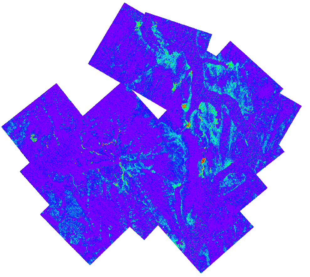ASTER TIR: (b10+b12+b13)/b11 + rainbow color table



  

This manipulation allowed me to highlight most representative pixels of the salt domes in red color.
If we look at the TIR (12 11 13) image we can see that the salt domes stand out in red or magenta, however, they all have different tinges, so choosing domes for my regions of interest I tried to incorporate all different shades of magenta to see if their spectra differ.
The image below on the right is a thermal  infra-red image of a section of Axel Heiberg Island with all the regions of interest marked by numbers 1- 9. And the image below on the left illustrates one of the ROIs which was drawn on the biggest salt dome of Axel Heiberg.

ASTER TIR: R:b12 G:b11 B:b13

 

Round Salt Dome ROI (most representative pixels)

Once all the nine ROIs were chosen I was able visualize them all on one graph allowing the comparison of the mean values of each of the five bands for each region of interest.



Just looking at the graph above I can see that most of the spectra have a very similar shape.There is a deep absorption feature in band 11 (second band of the TIR) and this is where most variability occurs. Only two regions of interest had a different shape of spectra: # 1 and #9, in spite of the fact that they also were highlighted as magenta in the TIR image.

Next step is running Spectral Analyst tool in order to compare our spectra to the spectral libraries.
I used two spectral libraries: ASUs_wasrds_rocks to ASTER TIR for identifying rock types and ASU mineral ASTER TIR for mineral identification created by the Arizona State University.

Comparing spectral signatures of #1 and #9 to the rock library showed that they are not similar to Rock Gypsum, but resemble much more the spectrum of Arkose (type of sandstone - silica rich) as illustrated below.


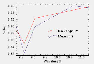
Comparison of all other ROIs to the rock spectral libraries produced the following results: Rock Gypsum or Rock Anhydrite as shown below.


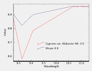
While comparison to the mineral libraries gave the following results: Gypsum or Gypsum var. Alabaster.


Of course this method is not very precise as the spectral resolution of ASTER images is 90m, however, it is a good approximation and it proves that the areas highlighted in magenta on the TIR ASTER images are indeed salt domes and are more specifically, most likely, gypsum.